
はじめに
この記事では、書籍『Kaggleで勝つデータ分析の技術』の第1章「分析コンペに必要なタスク」をもとに、住宅価格予測の実例を通して、Kaggleで役立つ実践的な手順を解説していきます。
E資格を取得された方々は、機械学習や深層学習の理論を体系的に学ばれたと思います。次に求められるのは、実データを使った分析力と、実践で通用するモデリングスキルです。Kaggleは、まさにそのスキルを磨くのに最適な環境だと言えるでしょう。
本記事では、scikit-learn に内蔵されている California Housing Dataset を使用し、住宅価格を予測する回帰モデルを構築します。通常はコンペのデータセットを用いるのですが、今回は、導入部の解説ということもあり、Kaggleのイメージを掴んでいただくために、擬似的なデータセットを使って解説したいと思います。
具体的には、このデータセットを訓練データ(train)としてモデルを学習し、その後、未知のテストデータ(test)に対して住宅価格(test_y)を予測します。
このような「教師あり学習による予測タスク」は、Kaggle などのデータ分析コンペティションでもよく出題されます。参加者は、テストデータの y(目的変数)をどれだけ正確に予測できるかを競い合い、モデル構築の実力を磨いていきます。

第1章のキーワード
| セクション | 重要語句(キーワード) |
|---|---|
| タスク理解 | タスクの概要/データの内容/予測対象 |
| データ理解(EDA) | カラムの型/値の分布/欠損値/外れ値(LOF)/相関・関係性 |
| 統計量 | 平均/標準偏差/最大・最小値/分位点/カテゴリ数/欠損数/相関係数 |
| 可視化 | 棒グラフ/箱ひげ図/バイオリンプロット/散布図/折れ線グラフ/ヒートマップ/ヒストグラム/Q–Qプロット/t-SNE/UMAP |
| 特徴量作成 | モデル学習用変換 |
| モデル作成 | GBDT/XGBoost/LightGBM |
| モデル評価 | クロスバリデーション(k-fold CV) |
| モデルチューニング | ハイパーパラメータチューニング/グリッドサーチ/ランダムサーチ |
タスク理解
分析コンペで成果を上げるための第一歩は、「どのような問題を解くのか」を明確に理解することです。今回は、California Housing Dataset を用いて、地域ごとの住宅の特徴量(例えば平均部屋数、築年数、世帯数、緯度経度など)から住宅価格(SalePrice)を予測するタスクを扱います。
住宅価格予測のタスクでは、与えられた住宅の特徴から、販売価格を予測することが求められます。 ここでは、scikit-learn内蔵の California Housing Dataset を使用します。
このように、目的変数と使用可能な変数を明確に洗い出すことで、
タスクのゴールと分析の出発点をしっかり定義することができます。

from sklearn.datasets import fetch_california_housing
import pandas as pd

housing = fetch_california_housing(as_frame=True)
df = housing.frame.copy()
df.head()
df.rename(columns={"MedHouseVal": "SalePrice"}, inplace=True)
df.head()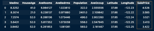
California Housing Datasetの主要な特徴量(説明変数)
| 列名(変数名) | 意味・説明 | 備考 |
|---|---|---|
SalePrice | 地域の住宅価格の中央値 | 元データでは MedHouseVal、単位は10万ドル |
MedInc | 地域の中央値収入(Median Income) | 数値は10,000ドル単位 |
HouseAge | 築年数 | 建物の築年数 |
AveRooms | 世帯あたりの平均部屋数 | 部屋数 / 世帯数 |
AveBedrms | 世帯あたりの平均寝室数 | 寝室数 / 世帯数 |
Population | 地域の総人口 | 各ブロック単位の人口合計 |
AveOccup | 世帯あたりの平均居住人数 | 総人口 / 世帯数 |
Latitude | 緯度 | 地理的特徴(北緯) |
Longitude | 経度 | 地理的特徴(西経) |
EDA(探索的データ分析)
EDA(探索的データ分析)は、モデルを構築する前にデータの構造や品質を深く理解するための重要なステップです。この段階で得られる知見は、後の前処理、特徴量の設計、モデル選定に大きく役立ちます。
- データ型の確認
各列(特徴量)のデータ型を調べることで、数値型かカテゴリ型かを判別します。これにより、それぞれに適した前処理方法(スケーリング、エンコーディングなど)を判断できます。 - 欠損値の確認
欠損している値があるかどうかを確認し、必要に応じて補完(例:平均値、中央値)や除去の処理を検討します。欠損値の扱い方によって、モデルの精度や安定性が大きく変わることがあります。 - 外れ値の検出(LOF)
Local Outlier Factor(LOF)アルゴリズムを使って、極端な値を持つデータ(外れ値)を特定します。これにより、モデルの学習に悪影響を与えるノイズを取り除く、または特別な扱いをする判断がしやすくなります。
# データ型確認
print(df.dtypes)

# 欠損値確認
print(df.isnull().sum())

# 外れ値検出(AveRoomsとSalePrice)
from sklearn.neighbors import LocalOutlierFactor
lof = LocalOutlierFactor(n_neighbors=20)
df['outlier_flag'] = lof.fit_predict(df[['AveRooms', 'SalePrice']])
MedInc float64
HouseAge float64
AveRooms float64
AveBedrms float64
Population float64
AveOccup float64
Latitude float64
Longitude float64
SalePrice float64
dtype: object
MedInc 0
HouseAge 0
AveRooms 0
AveBedrms 0
Population 0
AveOccup 0
Latitude 0
Longitude 0
SalePrice 0
dtype: int64統計量による把握
このステップでは、データの数値的な特徴を把握することが目的です。基本統計量や相関係数を確認することで、データのばらつきや中心傾向、外れ値の有無などを数値で理解できます。
.describe() を使うと、各特徴量の平均・標準偏差・最小値・最大値・四分位数などの統計情報を一覧で確認できます。これにより、変数ごとのスケールや異常値の兆しをつかむことができます。
さらに、.corr() を用いることで、相関係数を算出できます。これにより、目的変数である SalePrice と各特徴量との間に、どの程度の線形的な関係があるかを把握できます。相関が高い特徴量は、モデルの予測精度向上に役立つ可能性があるため、特徴量選択や重要度分析の参考になります。
# 基本統計量
print(df.describe())

# 相関係数
print(df.corr()['SalePrice'].sort_values(ascending=False))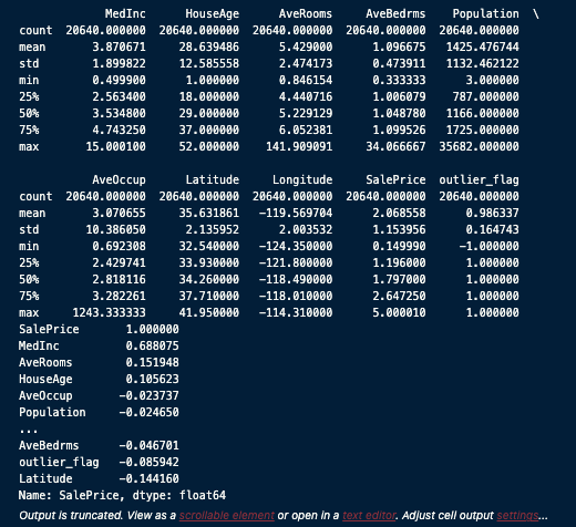
可視化による洞察
このステップでは、変数の分布や関係性を視覚的に捉えることを目的としています。統計量だけでは見えにくいパターンや異常値を、グラフを通して発見するためです。
たとえば、sns.scatterplot() を使うと、特徴量(例:AveRooms)と目的変数(SalePrice)との関係を散布図で表示できます。これにより、データの傾向が線形か非線形か、外れ値が存在するかなどを直感的に把握できます。
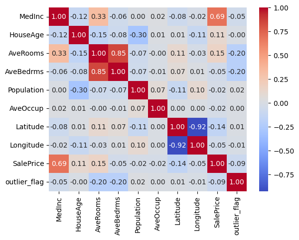
また、sns.heatmap() を使って相関行列のヒートマップを表示すると、複数の数値変数間の相関関係を色の濃淡で確認できます。相関が強い変数同士を簡単に見つけられるため、特徴量選択のヒントになります。
このような可視化は、後の特徴量エンジニアリングやモデル構築の方向性を決めるうえで、非常に重要な手がかりを与えてくれます。
import seaborn as sns
import matplotlib.pyplot as plt

# 散布図
sns.scatterplot(x='AveRooms', y='SalePrice', data=df)
plt.show()

# 相関ヒートマップ
sns.heatmap(df.corr(), annot=True, cmap="coolwarm", fmt=".2f")
plt.show()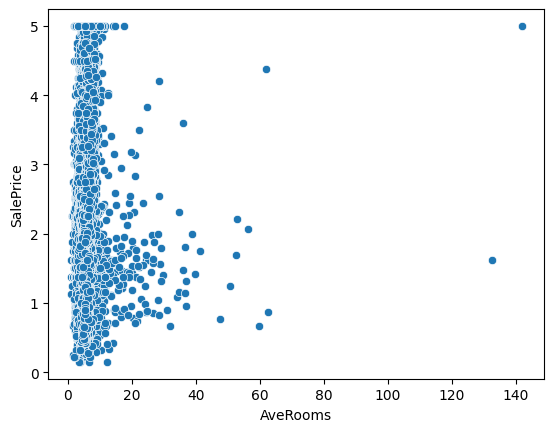
特徴量作成
このステップでは、モデルがより効果的に学習できるように、データの加工や変換を行います。なかでも「特徴量作成」は、モデルの性能に直結する非常に重要な工程であり、コンペティションでも勝敗を分けるポイントとなります。
たとえば、AveRooms や Population などの分布に歪みがある数値変数に対しては、log1p(対数変換)を適用することで、外れ値や極端な値の影響を和らげることができます。
このような変換によって、モデルは安定して学習しやすくなり、過学習のリスクを抑える効果も期待できます。結果として、より汎化性能の高いモデル構築につながります。
import numpy as np

# 対数変換(歪度の高い特徴量)
df['AveRooms_log'] = np.log1p(df['AveRooms'])
df['Population_log'] = np.log1p(df['Population'])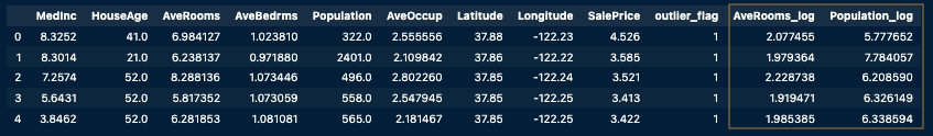
モデル作成(LightGBM)
このステップでは、LightGBM を使って、住宅価格を予測する回帰モデルを構築します。
LightGBMは、勾配ブースティングに基づく高速かつ高精度な機械学習ライブラリで、Kaggleをはじめとする多くの実践的なコンペティションでも定番のアルゴリズムです。
まずは、目的変数(SalePrice)と特徴量(説明変数)を分離し、train_test_split を使ってデータをトレーニング用とバリデーション用に分割します。
次に、LightGBMが扱いやすい形式である lgb.Dataset にデータを変換します。
その後、lgb.train() 関数を使ってモデルを学習させます。このとき、early_stopping_rounds を指定することで、一定回数スコアが改善しなければ学習を自動で停止させ、過学習のリスクを抑えることができます。
こうして構築したモデルは、バリデーションデータに対して初期的な予測精度を確認することができ、次のチューニングステップへの指針となります。
- LightGBMドキュメント
import lightgbm as lgb
from sklearn.model_selection import train_test_split

X = df.drop(['SalePrice', 'outlier_flag'], axis=1)
y = df['SalePrice']
X_train, X_val, y_train, y_val = train_test_split(X, y, test_size=0.2, random_state=42)

train_data = lgb.Dataset(X_train, label=y_train)
val_data = lgb.Dataset(X_val, label=y_val)

params = {'objective': 'regression', 'metric': 'rmse'}

# early_stopping_rounds は lgb.train の直接の引数ではなく、callbacks を使用します
callbacks = [lgb.early_stopping(stopping_rounds=50)]
model = lgb.train(params, train_data, valid_sets=[val_data], callbacks=callbacks)
[LightGBM] [Info] Auto-choosing row-wise multi-threading, the overhead of testing was 0.000367 seconds.
You can set `force_row_wise=true` to remove the overhead.
And if memory is not enough, you can set `force_col_wise=true`.
[LightGBM] [Info] Total Bins 2348
[LightGBM] [Info] Number of data points in the train set: 16512, number of used features: 10
[LightGBM] [Info] Start training from score 2.071947
Training until validation scores don't improve for 50 rounds
Did not meet early stopping. Best iteration is:
[100] valid_0's rmse: 0.463517モデル評価(クロスバリデーション)
このステップでは、KFold(交差検証)を使って、モデルの汎化性能(未知データへの対応力)を評価します。
交差検証とは、データを複数の分割(fold)に分けて、そのうちの1つを検証用、残りを訓練用として繰り返しモデルを学習・評価する方法です。
具体的には、KFold(n_splits=5) を使ってデータを5分割し、5回の学習と評価を実施します。
各イテレーションでは:
- LightGBM モデルを学習させ、
- 検証データに対して予測を行い、
- RMSE(平均二乗誤差の平方根)を計算して保存します。
最後に、5回分の RMSE の平均値を算出することで、全体としての予測性能を評価します。
このように交差検証を行うことで、特定のデータ分割に依存しない、より安定した評価指標を得ることができ、モデルの信頼性を高めることができます。
from sklearn.model_selection import KFold

kf = KFold(n_splits=5, shuffle=True, random_state=42)
rmse_list = []

for train_idx, val_idx in kf.split(X):
    tr_data = lgb.Dataset(X.iloc[train_idx], label=y.iloc[train_idx])
    va_data = lgb.Dataset(X.iloc[val_idx], label=y.iloc[val_idx])
    # verbose_eval 引数は callbacks で制御するため削除
    model = lgb.train(params, tr_data, valid_sets=[va_data], callbacks=callbacks)
    pred = model.predict(X.iloc[val_idx])
    rmse = np.sqrt(np.mean((pred - y.iloc[val_idx]) ** 2))
    rmse_list.append(rmse)

print("平均RMSE:", np.mean(rmse_list))
[LightGBM] [Info] Auto-choosing col-wise multi-threading, the overhead of testing was 0.000858 seconds.
You can set `force_col_wise=true` to remove the overhead.
[LightGBM] [Info] Total Bins 2348
[LightGBM] [Info] Number of data points in the train set: 16512, number of used features: 10
[LightGBM] [Info] Start training from score 2.071947
Training until validation scores don't improve for 50 rounds
Did not meet early stopping. Best iteration is:
[100] valid_0's rmse: 0.463517
[LightGBM] [Info] Auto-choosing row-wise multi-threading, the overhead of testing was 0.000193 seconds.
You can set `force_row_wise=true` to remove the overhead.
And if memory is not enough, you can set `force_col_wise=true`.
[LightGBM] [Info] Total Bins 2348
[LightGBM] [Info] Number of data points in the train set: 16512, number of used features: 10
[LightGBM] [Info] Start training from score 2.061298
Training until validation scores don't improve for 50 rounds
Did not meet early stopping. Best iteration is:
[100] valid_0's rmse: 0.466814
[LightGBM] [Info] Auto-choosing row-wise multi-threading, the overhead of testing was 0.000181 seconds.
You can set `force_row_wise=true` to remove the overhead.
And if memory is not enough, you can set `force_col_wise=true`.
[LightGBM] [Info] Total Bins 2347
[LightGBM] [Info] Number of data points in the train set: 16512, number of used features: 10
[LightGBM] [Info] Start training from score 2.070602
Training until validation scores don't improve for 50 rounds
Did not meet early stopping. Best iteration is:
...
Training until validation scores don't improve for 50 rounds
Did not meet early stopping. Best iteration is:
[100] valid_0's rmse: 0.47526
平均RMSE: 0.4652268869297102モデルチューニング(GridSearchCV)
このステップでは、GridSearchCV(グリッドサーチ)を使って、LightGBMモデルのハイパーパラメータ最適化を行います。
ハイパーパラメータとは、モデルの構造や学習方法を制御する設定値であり、その選び方によってモデルの性能は大きく変わります。
まず、param_grid にてチューニング対象のパラメータ(例:num_leaves、learning_rate、n_estimatorsなど)の候補値を定義します。
次に、GridSearchCV を用いて、これらのパラメータのすべての組み合わせに対して交差検証を実施し、最も良いスコアを出すパラメータセットを見つけます。
評価指標には scoring='neg_root_mean_squared_error' を指定します。これは RMSE(平均二乗誤差の平方根)を最小化することが目的ですが、scikit-learnでは最小化したいスコアは符号を反転(負の値)させて最大化問題として扱います。
こうして見つけた最適なハイパーパラメータは、最終的なモデルの学習やテストデータの予測に活用されます。
from sklearn.model_selection import GridSearchCV
from lightgbm import LGBMRegressor

param_grid = {
    'num_leaves': [31, 63],
    'learning_rate': [0.01, 0.1],
    'n_estimators': [100, 500]
}

grid = GridSearchCV(LGBMRegressor(), param_grid, cv=3, scoring='neg_root_mean_squared_error')
grid.fit(X_train, y_train)

print("ベストパラメータ:", grid.best_params_)
print("CV RMSE:", -grid.best_score_)
[LightGBM] [Info] Auto-choosing col-wise multi-threading, the overhead of testing was 0.000235 seconds.
You can set `force_col_wise=true` to remove the overhead.
[LightGBM] [Info] Total Bins 2347
[LightGBM] [Info] Number of data points in the train set: 11008, number of used features: 10
[LightGBM] [Info] Start training from score 2.064393
[LightGBM] [Info] Auto-choosing row-wise multi-threading, the overhead of testing was 0.000117 seconds.
You can set `force_row_wise=true` to remove the overhead.
And if memory is not enough, you can set `force_col_wise=true`.
[LightGBM] [Info] Total Bins 2347
[LightGBM] [Info] Number of data points in the train set: 11008, number of used features: 10
[LightGBM] [Info] Start training from score 2.078156
[LightGBM] [Info] Auto-choosing row-wise multi-threading, the overhead of testing was 0.000108 seconds.
You can set `force_row_wise=true` to remove the overhead.
And if memory is not enough, you can set `force_col_wise=true`.
[LightGBM] [Info] Total Bins 2348
[LightGBM] [Info] Number of data points in the train set: 11008, number of used features: 10
[LightGBM] [Info] Start training from score 2.073292
[LightGBM] [Info] Auto-choosing row-wise multi-threading, the overhead of testing was 0.000084 seconds.
You can set `force_row_wise=true` to remove the overhead.
And if memory is not enough, you can set `force_col_wise=true`.
[LightGBM] [Info] Total Bins 2347
[LightGBM] [Info] Number of data points in the train set: 11008, number of used features: 10
[LightGBM] [Info] Start training from score 2.064393
[LightGBM] [Info] Auto-choosing col-wise multi-threading, the overhead of testing was 0.000302 seconds.
You can set `force_col_wise=true` to remove the overhead.
[LightGBM] [Info] Total Bins 2347
[LightGBM] [Info] Number of data points in the train set: 11008, number of used features: 10
[LightGBM] [Info] Start training from score 2.078156
[LightGBM] [Info] Auto-choosing row-wise multi-threading, the overhead of testing was 0.000088 seconds.
You can set `force_row_wise=true` to remove the overhead.
And if memory is not enough, you can set `force_col_wise=true`.
[LightGBM] [Info] Total Bins 2348
[LightGBM] [Info] Number of data points in the train set: 11008, number of used features: 10
[LightGBM] [Info] Start training from score 2.073292
[LightGBM] [Info] Auto-choosing col-wise multi-threading, the overhead of testing was 0.000338 seconds.
You can set `force_col_wise=true` to remove the overhead.
[LightGBM] [Info] Total Bins 2347
[LightGBM] [Info] Number of data points in the train set: 11008, number of used features: 10
[LightGBM] [Info] Start training from score 2.064393
[LightGBM] [Info] Auto-choosing col-wise multi-threading, the overhead of testing was 0.000396 seconds.
You can set `force_col_wise=true` to remove the overhead.
[LightGBM] [Info] Total Bins 2347
[LightGBM] [Info] Number of data points in the train set: 11008, number of used features: 10
[LightGBM] [Info] Start training from score 2.078156
[LightGBM] [Info] Auto-choosing col-wise multi-threading, the overhead of testing was 0.000302 seconds.
You can set `force_col_wise=true` to remove the overhead.
[LightGBM] [Info] Total Bins 2348
[LightGBM] [Info] Number of data points in the train set: 11008, number of used features: 10
[LightGBM] [Info] Start training from score 2.073292
[LightGBM] [Info] Auto-choosing col-wise multi-threading, the overhead of testing was 0.000248 seconds.
You can set `force_col_wise=true` to remove the overhead.
[LightGBM] [Info] Total Bins 2347
[LightGBM] [Info] Number of data points in the train set: 11008, number of used features: 10
[LightGBM] [Info] Start training from score 2.064393
[LightGBM] [Info] Auto-choosing row-wise multi-threading, the overhead of testing was 0.000087 seconds.
You can set `force_row_wise=true` to remove the overhead.
And if memory is not enough, you can set `force_col_wise=true`.
[LightGBM] [Info] Total Bins 2347
[LightGBM] [Info] Number of data points in the train set: 11008, number of used features: 10
[LightGBM] [Info] Start training from score 2.078156
[LightGBM] [Info] Auto-choosing col-wise multi-threading, the overhead of testing was 0.000308 seconds.
You can set `force_col_wise=true` to remove the overhead.
[LightGBM] [Info] Total Bins 2348
[LightGBM] [Info] Number of data points in the train set: 11008, number of used features: 10
[LightGBM] [Info] Start training from score 2.073292
[LightGBM] [Info] Auto-choosing col-wise multi-threading, the overhead of testing was 0.000232 seconds.
You can set `force_col_wise=true` to remove the overhead.
[LightGBM] [Info] Total Bins 2347
[LightGBM] [Info] Number of data points in the train set: 11008, number of used features: 10
[LightGBM] [Info] Start training from score 2.064393
[LightGBM] [Info] Auto-choosing col-wise multi-threading, the overhead of testing was 0.000308 seconds.
You can set `force_col_wise=true` to remove the overhead.
[LightGBM] [Info] Total Bins 2347
[LightGBM] [Info] Number of data points in the train set: 11008, number of used features: 10
[LightGBM] [Info] Start training from score 2.078156
[LightGBM] [Info] Auto-choosing col-wise multi-threading, the overhead of testing was 0.000193 seconds.
You can set `force_col_wise=true` to remove the overhead.
[LightGBM] [Info] Total Bins 2348
[LightGBM] [Info] Number of data points in the train set: 11008, number of used features: 10
[LightGBM] [Info] Start training from score 2.073292
[LightGBM] [Info] Auto-choosing col-wise multi-threading, the overhead of testing was 0.000432 seconds.
You can set `force_col_wise=true` to remove the overhead.
[LightGBM] [Info] Total Bins 2347
[LightGBM] [Info] Number of data points in the train set: 11008, number of used features: 10
[LightGBM] [Info] Start training from score 2.064393
[LightGBM] [Info] Auto-choosing col-wise multi-threading, the overhead of testing was 0.000294 seconds.
You can set `force_col_wise=true` to remove the overhead.
[LightGBM] [Info] Total Bins 2347
[LightGBM] [Info] Number of data points in the train set: 11008, number of used features: 10
[LightGBM] [Info] Start training from score 2.078156
[LightGBM] [Info] Auto-choosing col-wise multi-threading, the overhead of testing was 0.000254 seconds.
You can set `force_col_wise=true` to remove the overhead.
[LightGBM] [Info] Total Bins 2348
[LightGBM] [Info] Number of data points in the train set: 11008, number of used features: 10
[LightGBM] [Info] Start training from score 2.073292
[LightGBM] [Info] Auto-choosing col-wise multi-threading, the overhead of testing was 0.000275 seconds.
You can set `force_col_wise=true` to remove the overhead.
[LightGBM] [Info] Total Bins 2347
[LightGBM] [Info] Number of data points in the train set: 11008, number of used features: 10
[LightGBM] [Info] Start training from score 2.064393
[LightGBM] [Info] Auto-choosing row-wise multi-threading, the overhead of testing was 0.000091 seconds.
You can set `force_row_wise=true` to remove the overhead.
And if memory is not enough, you can set `force_col_wise=true`.
[LightGBM] [Info] Total Bins 2347
[LightGBM] [Info] Number of data points in the train set: 11008, number of used features: 10
[LightGBM] [Info] Start training from score 2.078156
[LightGBM] [Info] Auto-choosing col-wise multi-threading, the overhead of testing was 0.000427 seconds.
You can set `force_col_wise=true` to remove the overhead.
[LightGBM] [Info] Total Bins 2348
[LightGBM] [Info] Number of data points in the train set: 11008, number of used features: 10
[LightGBM] [Info] Start training from score 2.073292
[LightGBM] [Info] Auto-choosing col-wise multi-threading, the overhead of testing was 0.000298 seconds.
You can set `force_col_wise=true` to remove the overhead.
[LightGBM] [Info] Total Bins 2347
[LightGBM] [Info] Number of data points in the train set: 11008, number of used features: 10
[LightGBM] [Info] Start training from score 2.064393
[LightGBM] [Info] Auto-choosing col-wise multi-threading, the overhead of testing was 0.000419 seconds.
You can set `force_col_wise=true` to remove the overhead.
[LightGBM] [Info] Total Bins 2347
[LightGBM] [Info] Number of data points in the train set: 11008, number of used features: 10
[LightGBM] [Info] Start training from score 2.078156
[LightGBM] [Info] Auto-choosing col-wise multi-threading, the overhead of testing was 0.000441 seconds.
You can set `force_col_wise=true` to remove the overhead.
[LightGBM] [Info] Total Bins 2348
[LightGBM] [Info] Number of data points in the train set: 11008, number of used features: 10
[LightGBM] [Info] Start training from score 2.073292
[LightGBM] [Info] Auto-choosing col-wise multi-threading, the overhead of testing was 0.000319 seconds.
You can set `force_col_wise=true` to remove the overhead.
[LightGBM] [Info] Total Bins 2348
[LightGBM] [Info] Number of data points in the train set: 16512, number of used features: 10
[LightGBM] [Info] Start training from score 2.071947
ベストパラメータ: {'learning_rate': 0.1, 'n_estimators': 500, 'num_leaves': 31}
CV RMSE: 0.4588566649776021テストデータに対する予測と提出ファイルの作成
このステップでは、学習済みのモデルを使って未知のテストデータに対する予測を行い、その結果を Kaggleに提出可能な形式のCSVファイルとして出力します。
実際のKaggleコンペティションでは、test.csv というファイルが提供されており、train.csv と同じ構造の特徴量を持っています。今回はこれを模して、学習時に使用したバリデーションデータ(X_val)を仮のテストデータとして利用します。
予測には、GridSearchCV で得られた最適なモデル(grid.best_estimator_)を使用します。このモデルで X_val に対する予測値を生成します。
そして、予測結果を Id カラムとともに DataFrame にまとめ、submission.csv という名前で保存します。この形式がそのままKaggleに提出できるスタイルです。
ここで紹介するのは擬似的な例ですが、実際のKaggleでは test.csv を読み込んだうえで、Id カラムと予測対象のカラム(例:SalePrice)を組み合わせて提出用のファイルを作成します。
# (例)テストデータをシミュレーション(通常は pd.read_csv('test.csv') で読み込む)
test_data = X_val.copy()  # 仮にバリデーションデータをテストデータとする

# 最終モデルで予測
final_model = grid.best_estimator_  # GridSearch で得られた最適モデルを使用
test_pred = final_model.predict(test_data)

# Kaggle提出用のデータフレーム作成(Id列を仮置き)
submission = pd.DataFrame({
    'Id': test_data.index,
    'SalePrice': test_pred
})

# CSVとして保存(Kaggleではこのファイルを提出)
submission.to_csv('submission_.csv', index=False)
これでフォルダの中にsubmission_.csvファイルが出来上がりました。このデータセットはコンペのデータセットではありませんので、提出はしませんが、この出来上がったファイルをKaggleのコンペのページで「Submit to Competition」で提出を行い、「Leaderboard」で「Score」を競い合います。
次回予告
分析コンペでは、構造化されたワークフローを繰り返し実践することが、精度向上のカギとなります。
とくに、EDA(探索的データ分析)や特徴量エンジニアリングの工夫は、モデルの予測精度に大きな影響を与える重要なポイントです。
ぜひ本記事の内容を参考に、Kaggleでの実践やご自身のプロジェクトにチャレンジしてみてください。
次回の第2章では、分析コンペにおける「タスクと評価指標」の考え方について詳しく解説します。
どのようなタスク(分類・回帰など)が存在し、どの評価指標が用いられるのかを理解することで、より戦略的にアプローチできるようになります。

コメント